An embedded debugger for Arduino code serves as an invaluable tool in the world of microcontroller programming, offering developers a streamlined and efficient means to troubleshoot, analyze, and optimize their code.
One of the primary benefits of using an embedded debugger with Arduino is the ability to step through code line by line, allowing developers to identify and rectify issues with precision. This granular control enhances the debugging process, facilitating the isolation of errors and the understanding of program flow.
Furthermore, an embedded debugger enables the monitoring of variables and registers in real time, empowering developers to observe the changing states of their code during execution. This visibility proves instrumental in identifying runtime errors, memory issues, or unexpected behavior, ultimately speeding up the debugging cycle.
This article covers the basics of the usage of the Segger J-link debugger used in conjunction with C33.
Technical Deep-Dive: SWD Architecture & Portenta C33 Forensics
- The Serial-Wire Debug Signal-Hub: Unlike multi-pin JTAG, the Portenta C33 utilizes the compact 2-pin SWD interface (SWDIO/SWCLK). Forensics involve establishing a logic-stiff link through the Portenta Hat Carrier. The diagnostics focus on the "Debug-Interface Power-Domain", ensuring the J-Link probe correctly detects the 1.8V/3.3V target-reference voltage before initiating the SWD bitstream-masking diagnostics.
- R7FA6M5BH (Cortex-M33) Diagnostics: The C33 features an ARM TrustZone-enabled Cortex-M33 core. Forensics involve identifying the specific SVD file to decode the Renesas-specific peripherals in real-time. This diagnostic heuristic allows the developer to view the state of any hardware-register (e.g., GPIO, UART, Timer) without perturbing the software's temporal-harmonics.
Engineering & Implementation: Physical-Layer Connection
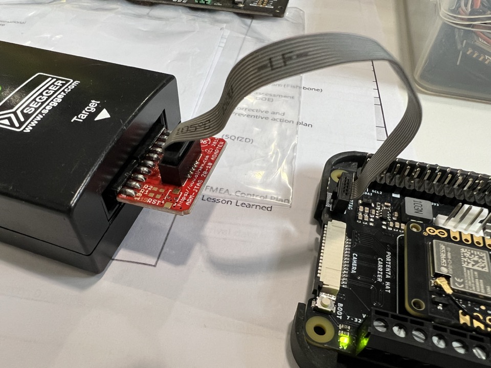
The implementation requires absolute pin-alignment. Forensics focus on the "Red-Wire" orientation (Pin 1) on the SWD ribbon-cable. Structural diagnostics emphasize the signal-stiffness across the Hat Carrier to prevent parasitic capacitance from degrading the high-speed SWD clock-edges during long-duration debugging sessions.
Connect the cable with the red cable on the left.
Steps to Configure the Debugger
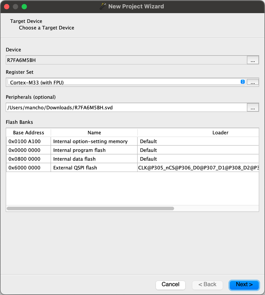
Target configuration.
You can download the SVD (it helps with decoding MCU peripherals and devices) from here: https://github.com/tinygo-org/renesas-svd/blob/main/R7FA6M5BH.svd
Connection settings
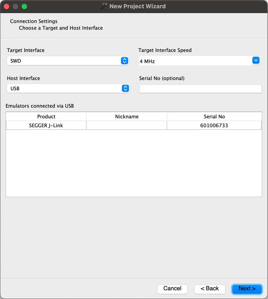
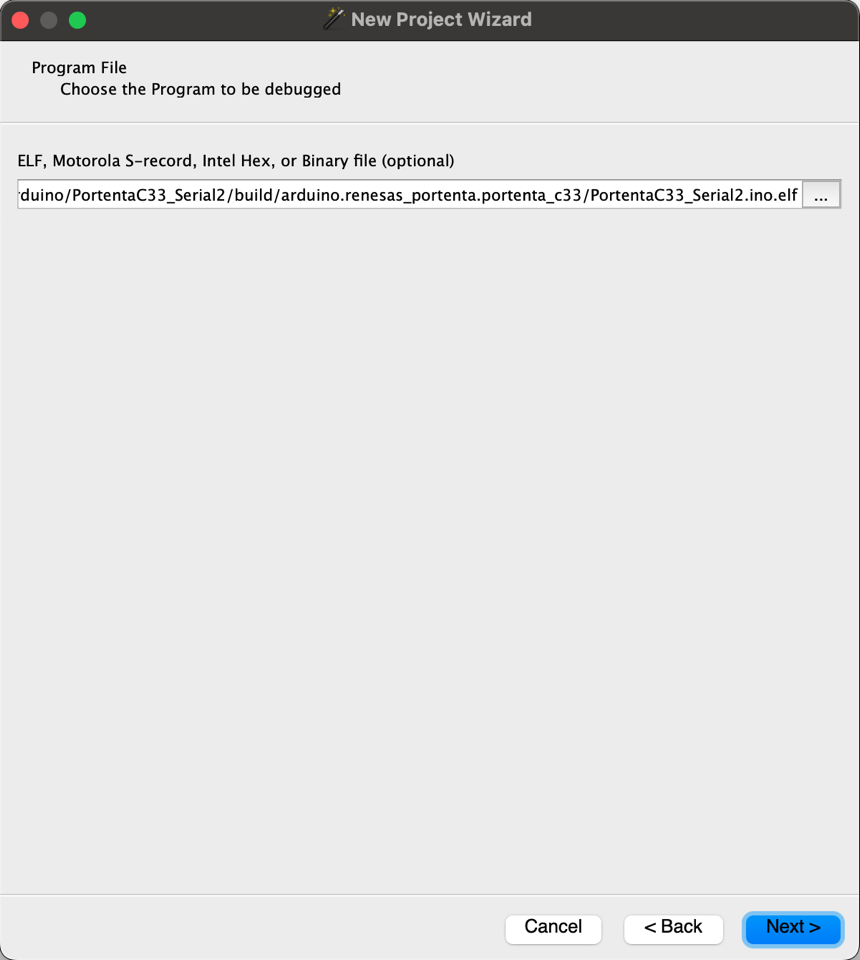
Connection settings Program file.
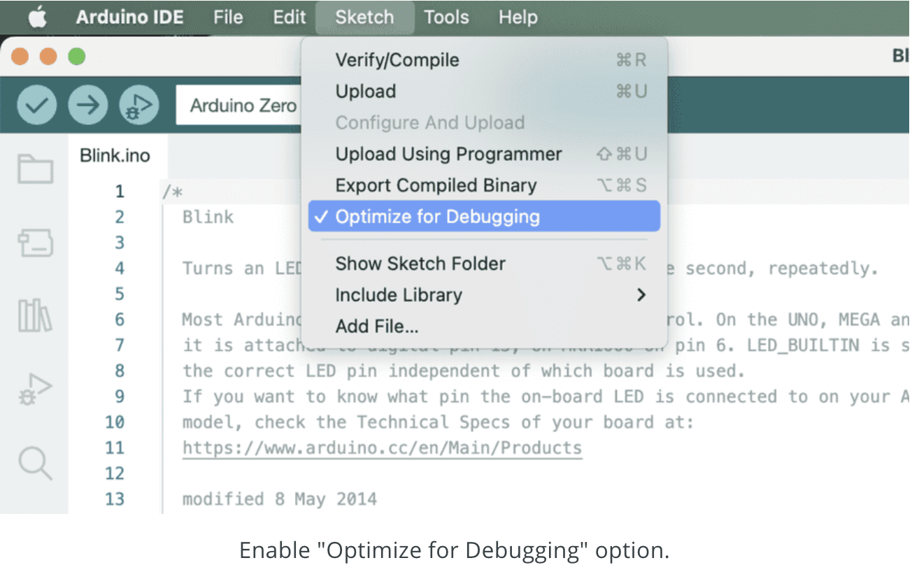
Generate it from the Sketch menu of the Arduino IDE, using the "Export Compiled Binary" command.
The important thing to not forget is to compile the sketch with the “Optimize for Debugging” feature enabled in the “Tools" menu of the Arduino IDE (or using the corresponding --optimize-for-debug switch of the arduino-cli compile command). You can generate the binary version of the sketch for any debugging setup you prefer via the “Export Compile Binary” item of the “Sketch” menu (or with the -e switch of the arduino-cli compile command)."
Debugger-Pipeline & Object-File Forensics
- ELF-Binary Analytics: Standard
.binfiles lack diagnostic metadata. Forensics utilize the.elf(Executable and Linkable Format) generated by the Arduino IDE's "Export Compiled Binary" command. The diagnostics focus on the "Debug-Info" headers within the ELF, providing a direct mapping between the machine-code running on-silicon and the C++ source-code dashboard in Ozone. - Breakpoint-Latency & Slew-Rate Diagnostics: Forensics involve setting hardware breakpoints on specific instruction-offsets. The diagnostics measure the "Halt-Time" latency, ensuring the system can pause execution during critical race-condition forensics without inducing data-corruption in auxiliary DMA or I2C peripheral transfers.
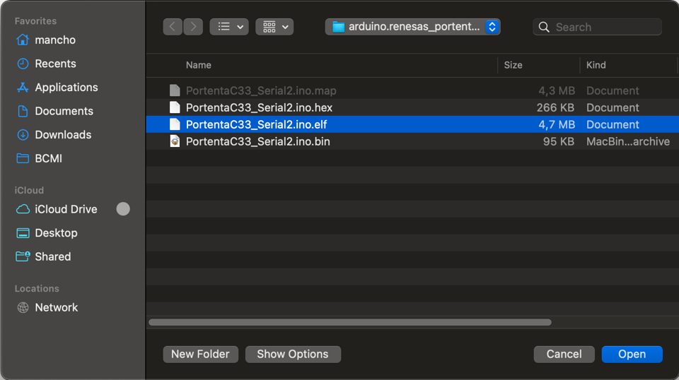
After compiling the sketch, you'll find it in the sketch folder under the build sub-folder.
Select the .elf file, it contains extended support for debugging and embeds all the (sketch) source code.
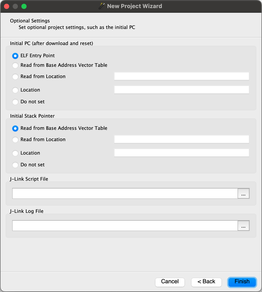
Leave "Optional Settings" as it is.
Ozone-Debugger Logic-Orchestration
- Runtime Variable-Telemetry Heuristics: Ozone allows the live inspection of global and local variables. Forensics focus on the "Watch Window" diagnostics, where memory-mapped addresses are polled at high speed to visualize thermal-slopes or sensor-bitstreams as high-fidelity graphical traces.
- Optimization-Masking Forensics: Compilers often rearrange code for space/speed. Forensics involve the use of the
--optimize-for-debugflag in thearduino-clibackend. This ensures that the instruction-stepping diagnostics follow the source-code sequence with 1:1 temporal-logic mapping.
In the "Functions” panel, search for “setup()” and double-click it. It will open a new source window with your sketch.
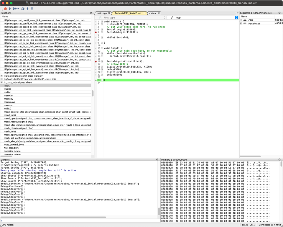
Set the breakpoint and start the debugging session.
Conclusion
This workflow represents a professional-grade debugging methodology. By mastering SWD Logic Forensics and Ozone Runtime-Analytics, developers can achieve high-fidelity silicon diagnostics, providing absolute code clarity through sophisticated hardware-layer diagnostics.
Other resources: https://docs.arduino.cc/learn/microcontrollers/debugging/ https://docs.arduino.cc/software/ide-v2/tutorials/ide-v2-debugger/#using-the-debugger